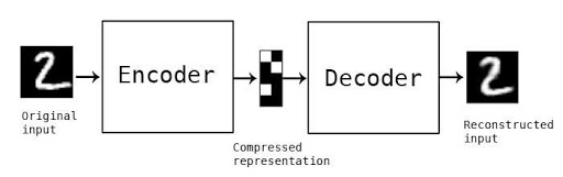
The process of transforming input x to latent representation z is called the encoder and from latent variable z to reconstructed version of the input![]() is referenced as the decoder.
is referenced as the decoder.
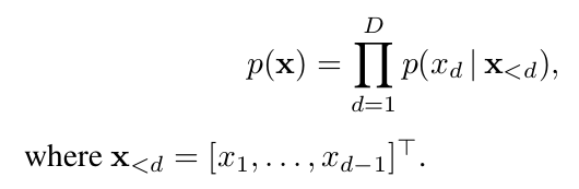
Let’s suppose we are given a training set of examples ![]() .Here
.Here ![]() and
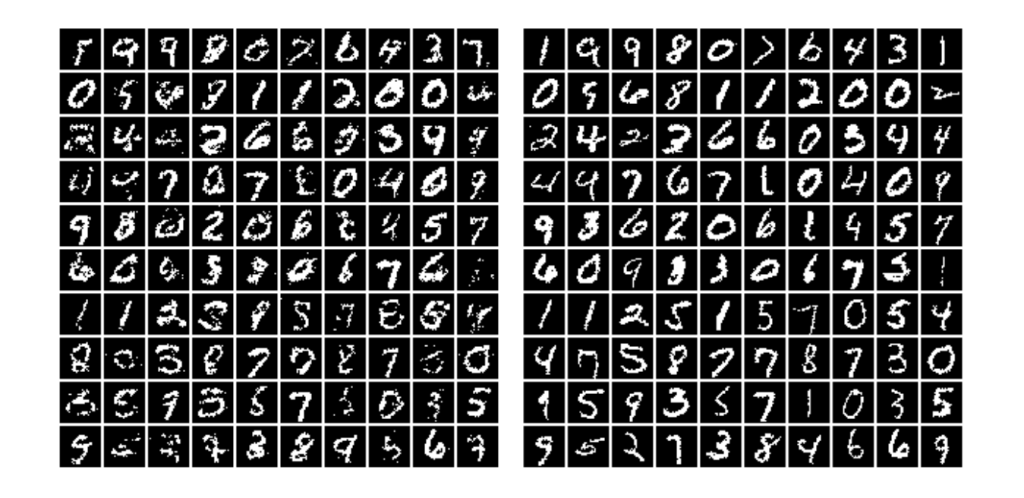
and ![]() , because we are concentrating on binary inputs. Our motivation is to learn a latent representation, by which we can obtain the distribution of these training examples using deep neural networks.
, because we are concentrating on binary inputs. Our motivation is to learn a latent representation, by which we can obtain the distribution of these training examples using deep neural networks.
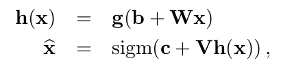
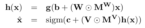
Suppose the model contains one hidden layer and tries to learn h(x) from its input x such that from it, we can generate reconstruction ![]() which is as close as possible to x. Such that,
which is as close as possible to x. Such that,
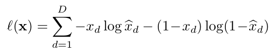
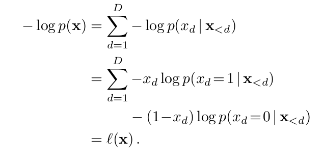
We can treat ![]() as the model’s probability that
as the model’s probability that ![]() is 1, so l(x) can be understood as a negative log-likelihood function. Now the autoencoder can be trained using a gradient descent optimization algorithm to get optimal parameters (W, V, b, c) and to estimate data distribution. But the loss function isn’t actually a proper log-likelihood function. The implied data distribution
is 1, so l(x) can be understood as a negative log-likelihood function. Now the autoencoder can be trained using a gradient descent optimization algorithm to get optimal parameters (W, V, b, c) and to estimate data distribution. But the loss function isn’t actually a proper log-likelihood function. The implied data distribution![]() isn’t normalized
isn’t normalized![]() . So outputs of the autoencoder can not be used to estimate density.
. So outputs of the autoencoder can not be used to estimate density.
Define![]() , and
, and![]() . So now the loss function in the previous part becomes a valid negative log-likelihood function.
. So now the loss function in the previous part becomes a valid negative log-likelihood function.
Here each output![]() must be a function taking as input
must be a function taking as input ![]() only and giving output the probability of observing value
only and giving output the probability of observing value ![]() at the
at the![]() dimension. Computing above NLL is equivalent to sequentially predicting each dimension of input x, so we are referring to this property as an autoregressive property.
dimension. Computing above NLL is equivalent to sequentially predicting each dimension of input x, so we are referring to this property as an autoregressive property.
Since output![]() must depend on the preceding inputs
must depend on the preceding inputs![]() , it means that there must be no computational path between output unit
, it means that there must be no computational path between output unit![]() and any of the input units
and any of the input units ![]()
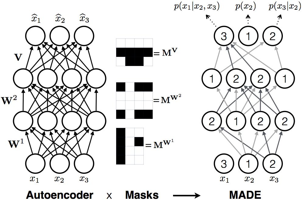
For every layer![]() , ml(k) stands for the maximum number of connected inputs of the kth unit in the lth layer. In above figure, value written in each node of MADE architecture represents ml(k).
, ml(k) stands for the maximum number of connected inputs of the kth unit in the lth layer. In above figure, value written in each node of MADE architecture represents ml(k).
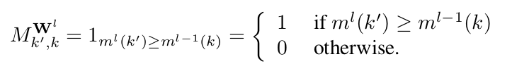
Where![]() ,
, ![]() and
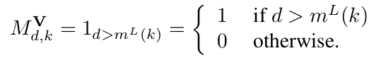
and![]() . Note that ≥ becomes > in output mask matrix. This thing is vital as we need to shift the connections by one. The first output x2 must not be connected to any nodes as it is not conditioned by any inputs.
. Note that ≥ becomes > in output mask matrix. This thing is vital as we need to shift the connections by one. The first output x2 must not be connected to any nodes as it is not conditioned by any inputs.
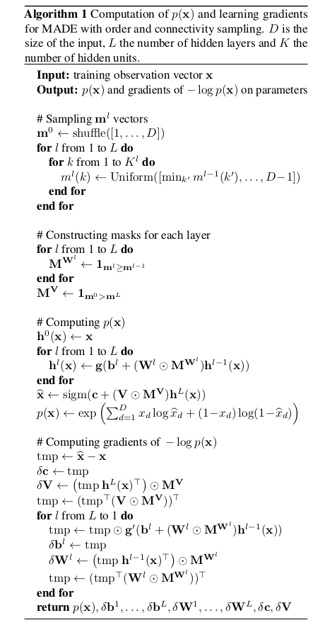
We set ml(k) for every layer![]() by sampling from a discrete uniform distribution defined on integers from mink’ ml-1(k’) to D-1 whereas m0 is obtained by randomly permuting the ordered vector [1,2,…,D].
by sampling from a discrete uniform distribution defined on integers from mink’ ml-1(k’) to D-1 whereas m0 is obtained by randomly permuting the ordered vector [1,2,…,D].
MV,W = MVMW1MW2…MWL represents the connectivity between inputs and outputs. Thus to demonstrate the autoregressive property, we need to show that MV,W is strictly lower diagonal, i.e. MV,Wd’,d is 0 if d'<=d.
Let’s look at an algorithm to implement MADE:
Essentially, the paper was written to estimate the distribution of the input data. The inference wasn’t explicitly mentioned in the paper. It turns out it’s quite easy, but a bit slow. The main idea (for binary data) is as follows:
- Randomly generate vector x, set i=1
- Feed x into autoencoder and generate outputs
 for the network, set p =
 .
. - Sample from a Bernoulli distribution with parameter p, set input xi = Bernoulli(p).
- Increment i and repeat steps 2-4 until i > D.
The inference in MADE is very slow, it isn’t an issue at training because we know all x<d to predict the probability at dth dimension. But at inference, we have to predict them one by one, without any parallelization