Flight Radar : Building your own simple, real time Flight Monitor using Python

Reading Time: 8 minutes

Flight Radar : Building your own simple, real time Flight Monitor using Python

Introduction

According to a previous year report, there were around 9728 planes – carrying about 1,270,406 people – in the sky at a given moment! How are all the flights controlled and avoided from colliding with each other? Well, there are complex systems which monitor real-time sky traffic and provide necessary details to the pilot. In case the projectiles of two or more flights meet, a warning system is activated and the necessary plan to escape the collision is provided.

The aim of this article is not to inform you about ATC processes, however, we would be using the data from the servers of ICAO to make our own simplistic Flight Radar.  Every aircraft in air is assigned its own ICAO 24-bit address. This unique address of an aircraft is then used to access some important information like the location (latitude, longitude), flight altitude and velocity.


Pre Requisites

  1. Basic knowledge of Python and handling of Jupyter Notebooks.
  2. Python, pip, and git installed on your machine.
  3. Working with the terminal.
  4. Libraries – Matplotlib, Basemap

If new to these points I advise you to look out for the Anaconda distribution. If you are on Windows, working with Anaconda Prompt is the best and easiest way to deal with development processes in python.

The basic requirement of our code is to fetch information from the ICAO 24 – bit address of each aircraft we care about. Well, there is a very simple and effective tool available for this. The Open Sky API! Just a call to this API will help us fetch the details of the aircraft we are looking for! 90% of the work done right?! That’s why I love APIs.


Installing required packages

Now I advise you to make a separate folder, where you’ll work.

Matplotlib

Flight Radar : Building your own simple, real time Flight Monitor using Python

If you have Anaconda distribution you’ll be already having matplotlib installed. Matplotlib is a powerful Python library for fantastic data visualizations. If you are interested and passionate about visualizations I advice you to take a separate tutorial on matplotlib (and seaborn).

If you don’t have anaconda installed, you can fetch the package from the Python Package Index (PyPI).

Just run the following in your terminal

pip install matplotlib

Matplotlib – Basemap

Flight Radar : Building your own simple, real time Flight Monitor using Python

Now we need Basemap. Basemap was developed by the same developers who had worked on matplotlib. Those were the years when python was being shaped into a multi-functional, easy to use, research-oriented language it is now. Ahh, the golden years of python!

Noo! Let’s not deviate!

Basemap offers easy integration with matplotlib, a very necessary function for our code to work. There are many other GIS specific great libraries in python but since we need integration with matplotlib ( and basemap is the only one I’ve worked with:) ) we will go with basemap. If you’re having conda it’s easy.

conda install -c anaconda basemap

If you do not have conda you need to clone the basemap github repository and then run setup.py

git clone https://github.com/matplotlib/basemap.git

Move to the directory where the repo is cloned and run

python setup.py install

Open-Sky Network API

Flight Radar : Building your own simple, real time Flight Monitor using Python

The API is not available on either conda cloud or PyPI and so it requires manual installation.

git clone https://github.com/openskynetwork/opensky-api.git
cd opensky-api/python
python setup.py install

High-Resolution Maps : Basemap (Optional)

By default, basemap has very minimalistic maps installed with it. However, if we really care about the deep details of our maps we should separately install high resolution maps. However this means our code will take more time to process since it requires to render such high detailed maps.


Let’s Code!

Flight Radar : Building your own simple, real time Flight Monitor using Python

Now let’s open up our Jupyter Notebooks and import the required packages. In the same directory where you’ve installed OpenSky API, open jupyter notebook by simply typing in

jupyter notebook

Importing requirements

import matplotlib.pyplot as plt
from opensky_api import OpenSkyApi
from mpl_toolkits.basemap import Basemap
from IPython import display

All the plots made by matplotlib are stored at a specific memory location while the code runs. When we run the code, it by default prints a message telling us where the plot is saved. However, if instead, we want all the plots to be displayed as soon as they are made inside our notebook we need to inform it explicitly.

%matplotlib inline

Now let’s define a function which will help us fetch the latitude and longitude of the flights (called states in OpenSky API documentation). Now by default, the OpenSky API returns the states of all the flights in contact with the ICAO servers. We do not want the details of all the flights in the sky. What we will do is define a box using latitude, longitude coordinates of its corners and fetch the data of only that box. This box will be over Indian Airspace. Hence we will fetch the details of flights only over Indian Airspace. Since it is a large area we will display the real-time movements of flights only in the region south of Tropic Of Cancer, which has some of the important Indian airports and also hosts many international flight routes.

The latitude, longitude coordinates can be easily known from Google Maps by clicking at random points within our desired box.

Let’s define a function which returns the latitude, longitude coordinates of the flights in the box specified.

def coordinates():
    api = OpenSkyApi()
    lon = []
    lat = []
    j = 0
    # bbox = (min latitude, max latitude, min longitude, max longitude)
    states = api.get_states(bbox=(8.27, 33.074, 68.4, 95.63))
    for s in states.states:
        lon.append([])
        lon[j] = s.longitude
        lat.append([])
        lat[j] = s.latitude
        j+=1
    return(lon, lat)

Here  api.get_states(…) helps us define the box under which we need to fetch the flights’ data. Here the bbox covers Indian Airspace. This code snippet is already commented and so it’s not difficult to understand. The loop iterates over all the states fetched from the bbox specified and we extract only the latitude and longitude out of it. At last, the (lat, lon) lists are returned which now possess the location of every flight over the Indian Airspace at the time you are reading this!

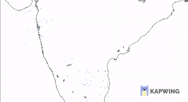
Now let’s plot the coordinates fetched on the Indian Airspace. As mentioned, to properly visualize the aircrafts’ movements over space we would consider only the region of Indian Airspace below the Tropic of Cancer.  

What we will do here is plot the map with the coordinates on it and then re-plot for a certain number of times. Every time a new plot is displayed, coordinates of flights are shown for the time when the API was called. Since there is some inherent time taken by the code to print the high-resolution map, the next time we fetch the data from the API, we receive updated coordinates. This will help us show the exact path of each aircraft.

To display the plots one after the other it’s obvious we will use an iteration and plot the map for every iteration. Let’s also ask the user the number of iterations he/she wants to make it a bit interactive.

print("How many Iterations?")
a = int(input())

Now let’s code the iteration.

for i in range(1, a + 1) :
    fig_size = plt.rcParams["figure.figsize"]
    fig_size[0] = 20
    fig_size[1] = 20
    plt.rcParams["figure.figsize"] = fig_size
    lon, lat = coordinates()
    m = Basemap(projection = 'mill', llcrnrlat = 8.1957,   urcrnrlat = 23.079, llcrnrlon = 68.933, urcrnrlon = 88.586, resolution = 'h')
    m.drawcoastlines()
    m.drawmapboundary(fill_color = '#FFFFFF')
    x, y = m(lon, lat)
    plt.scatter(x, y, s = 5)
    display.clear_output(wait=True)
    display.display(plt.gcf())

Let’s break down and understand this for – loop step by step

fig_size = plt.rcParams["figure.figsize"]
fig_size[0] = 20
fig_size[1] = 20
plt.rcParams["figure.figsize"] = fig_size

What this chunk of code does is set a size to the plot image displayed in the Jupyter Notebook. By default the size is insufficient for us to monitor all the flights.

lon, lat = coordinates()

This is pretty obvious. coordinates function is called and the lists with the values of flight latitudes and longitudes are stored in the lists lat and lon respectively.

m = Basemap(projection = 'mill', llcrnrlat = 8.1957,   urcrnrlat = 23.079, llcrnrlon = 68.933, urcrnrlon = 88.586, resolution = 'h')

This code segment creates a basic Basemap. In cartography, there are many projections available to choose from. The miller projection is the simplest form of flat maps that we generally see. If you want to read more about map projections you can do it here.

llcrnrlat is just an abbreviation to lower left corner latitude. What these 4 variables do is again define a region for which the map has to be generated. In this case, it is the Southern part of India. I have set the resolution to high (‘h’) to render really high-quality maps. If you think it uses a lot of compute you can switch to lower quality by setting resolution = ‘c’ instead.

m.drawcoastlines()
m.drawmapboundary(fill_color = '#FFFFFF')

I think this is pretty readable. It draws coastlines and boundary for the map and sets map color to white.

x, y = m(lon, lat)
plt.scatter(x, y, s = 5)

This segment at last prints the coordinates on the basemap. plt.scatter(…) is actually a matplotlib function. This is where the integration comes into the picture which we had discussed in the introduction paragraph. Both the basemaps and scatterplot we created are plotted on single axes providing us with the final map!

display.clear_output(wait=True)
display.display(plt.gcf())

As soon as the plot is generated and printed the next time a plot is generated we need to remove the previous plot and display the present one. This code does exactly the same thing and hence adds “motion“ to the flights plotted!

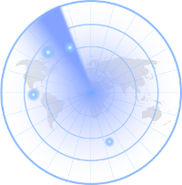
This is how the final plot looks like:

(look closely, this is a GIF which is exactly how your actual output will look like)

Flight Radar : Building your own simple, real time Flight Monitor using Python


Getting Started with Machine Learning with Python

Reading Time: 9 minutes

– BY AMAN PANDEY


In my previous tutorial Constructing a Simple Blockchain using PYTHON , I did promise on writing the further about Applications of Blockchain & their Implementation. I will soon post regarding the same. I wanted to make the next tutorial over Blockchain as simple as possible, so I will be needing some time to design my next Tutorial blog on Blockchain. So, keep patience :).

Now, alongside me learning the blockchain, I was also working on Machine Learning and Deep Learning, as if it is my core Learning subjects.

In my last blog on Blockchain, I received few comments that the terms were not easy to understand, thus making the blog difficult to read for the readers completely new to programming, which, is of course very true because these technologies have their own glossary.

I came up with an idea to give you guys the taste of the Machine Learning Models with the easiest way possible, to make my blog better, or you can say that I just trained myself ; P.

Getting Started with Machine Learning with Python

Machine Learning

“Machine learning is a field of computer science that uses statistical techniques to give computer systems the ability to “learn” with data, without being explicitly programmed.”

Does that help?

I guess not!

My belief for doing the things perfectly is by actually doing them.

I would love to dip my hands into something worthy rather than sitting and listening to some boring lectures (though they are not that boring, it’s my way of understanding things 😀 ;p).

So, here I present you the best way, that I think is well enough to get you guys a boost start in making and understanding machine learning models.

Getting Started

Before actually getting started, let’s get back to the definition and try to understand it,

“Machine learning is a field of computer science that uses statistical techniques to give computer systems the ability to “learn” with data, without being explicitly programmed.”

Few words to underline:

-statistical

-ability to “learn”

-without being explicitly programmed

Now in this tutorial, I will not be taking the names of any technical term except the ones that you need to know. Or better to say the ones which are extremely required. Because I think, for those who are having their first experience in Machine Learning, it becomes extremely confusing when such “Out of their Glossary” kind of terms starts bombarding on them.

So, now how can we start understanding above-underlined terms? How do we actually implement them? How a machine with zero IQ will learn? How will it answer to the problems that are new to them? And most importantly how will we train the machine?

I will try to explain it in very short as I can.

->Statistical means you have previously recorded data of Thousands or millions or even billions of records. E.g. the data of

  • Occurrences of words in emails marked as SPAM
  • Data of various houses & their degree of damage along with structural information of the houses etc.

These datasets are used to make a Mathematical Model, which will then be used to predict the answers for the test datasets.

->Ability to “learn” here is not that computer gets some human power or something and starts learning on its own. Naah. This the thing which we recently called the Mathematical Model.

We actually create a mathematical model using the previous datasets and train them on basis of them, or in other words to say we actually plot them using various techniques (in fancy words called as Machine Learning Algorithms ) based on features (another fancy term), which actually stands for various properties or information related to some object in which we are going to predict our results on.

E.g.

  • Linear Regression
  • Logistic Regression
  • Decision tree Classifier
  • Random Forest
  • Neural Networks etc. etc. etc.

😀 Haha.. none of them gives us clue what they mean. Right?

Now before moving forward I would love to illustrate you with some example, you’ll love the way it all works:

Suppose you want to distinguish between an “apple” and an “orange”.

Getting Started with Machine Learning with Python

Now what you have for information about them?

Ummm, maybe weight, or color may be different levels of its ripeness as it may be possible that apple or orange may have different weights and color at different ripeness level.

Isn’t it?

“Now, we have two features color and weight now.”

A mathematical model is created by plotting these properties on a 2d graph as shown. But that is possible if we have some numerical representation of a feature.

Getting Started with Machine Learning with Python

In this way, we plot them(intuitively), and ready to classify them.

So for the training data we will plot new inputs on this graph and the examples plotted on this graph having ordinates > line will be oranges and the ones having ordinates <line, are the apples.

This is an example of simple Linear regression, in which we plot a line to classify between two targets.

And this is how a computer performs without being explicitly programmed.

Why Python?

PYTHON being the most famous language of today, besides another like JAVASCRIPT, is extremely simple, ridiculously fast, and has a huge Library for various uses ranging from COMPUTATIONAL UTILITIES to CREATING A P2P network.

It may happen that you want to do Machine Learning, and you don’t need to take a full course on python. I know many of the sources where you can learn enough python to go on with machine learning.

Getting Started with Machine Learning with Python

Starting with Building a Machine Learning model.

Steps : –

    1. Installing required Libraries
      Pandas, scikit learn, numpy… that’s it for now
    2. Creating python file, importing required libraries and all
    3. Loading dataset
      we can do with any library but for now, we’ll just have Iris flower dataset, which is actually considered as “Hello world” dataset for python, you’ll find at many places
    4. Exploring our dataset
    5. Making our first model
    6. Printing the accuracy of our model
    7. Testing various models

**Note: Before starting anything I need you to clone the following repo from GitHub link to your local PC:

https://github.com/johnsoncarl/startingWithMachineLearning

1. Installing required Libraries

In the Github repo given above, you’ll find a file name required.txt, this file has all the requirements for the project, just run the following command into your terminal, being into repo directory to install required packages.

sudo apt-get -y install python3-pip
pip3 install -r required.txt

This will install all the required libraries for our model.

2. Creating a Python file, importing libraries and all

Create a python file of your desired name with .py extension in the repo directory, and open it into your favourite text editor and import required libraries as follows:

import pandas as pd
from sklearn import model_selection
from sklearn.metrics import accuracy_score
# these are various machine learning models already stored in the sklearn library
from sklearn.linear_model import LogisticRegression
from sklearn.tree import DecisionTreeClassifier
from sklearn.neighbors import KNeighborsClassifier
from sklearn.discriminant_analysis import LinearDiscriminantAnalysis
from sklearn.naive_bayes import GaussianNB
from sklearn.svm import SVC


3. Loading the Dataset

Here we shall use read_csv() function of pandas library to read our dataset as follows.

file = pd.read_csv("iris.data", header = None)
file.head(5)

file.head(5) will view the first 5 rows of the dataset.

And do notice, in read_csv we have header = None, this is used because our dataset does not contain any headings to define the columns. It will look something like this:

Getting Started with Machine Learning with Python

4. Exploring our dataset

Few things before building our model.

Run the following lines to print various information about the dataset we are going to use.

  1. Finding dimensions
print(file.shape)

 2. Describing data with analytics

print(file.describe())

3. Printing distribution of class(grouping according to column no 4, as we have seen in point 3.)

print(file.groupby(4).size())


5. Making our First model

Before making any Model and testing data on it, we have a very important step, that is to creating training & testing datasets separately. To train the model on and to test the model on.

For this purpose, we have already imported model_selection  from sklearn.

->  Splitting dataset into Training and Testing

Following code is to first change the dataset into a 2D array, then separating the target from it into Y, defining seed. And finally dividing our dataset into training and validation dataset.

array = file.values     # dataset to a 2d array
X = array[:,0:4]        # feature dataset
Y = array[:,4]          # target dataset
# validation size is used to take out 0.3 i.e 30% of our dataset into test dataset.
validation_size = 0.30
seed = 5                # why random seed is used its given
# finally slicing our dataset into training and testing
X_train, X_validation, Y_train, Y_validation = model_selection.train_test_split(X, Y, test_size=validation_size, random_state=seed)
# to test if its sliced properly
print(X_train[:3])

-> Defining and using our model

We will be using simple Logistic Regression classifier as our model and use to train our dataset and predict the outcomes.

Few steps, Define model, then fit model, then predict the output.

model = LogisticRegression()
# fitting our model
model.fit(X_train, Y_train)
# predicting outcomes
predictions = model.predict(X_validation)
print(predictions[:10])


print(predictions[:10])) will print the predictions on validation dataset after being train on the training dataset.

6. Printing the accuracy of our model

Now to rate our model we need to find its accuracy. For this, we need to compare our Validation data to our predicted data. And since we are using a library we don’t need to manually calculate it.  We have the following command to do this job as we have already imported accuracy_score from sklearn.metrics.

print(accuracy_score(Y_validation, predictions))


I had the following output when I ran this in my ipython notebook, which I have included in my Github repo.

Getting Started with Machine Learning with Python

It is 93.33% accurate.

And now, you are done with your first machine learning model.

7. Testing Various models

model = LogisticRegression()
model.fit(X_train, Y_train)
predictions = model.predict(X_validation)
print("Logistic Regression: ", accuracy_score(Y_validation, predictions, "\n"))
model = DecisionTreeClassifier()
model.fit(X_train, Y_train)
predictions = model.predict(X_validation)
print("DecisionTreeClassifier: ", accuracy_score(Y_validation, predictions, "\n"))
model = KNeighborsClassifier()
model.fit(X_train, Y_train)
predictions = model.predict(X_validation)
print("KNeigbhorsClassifier: ", accuracy_score(Y_validation, predictions, "\n"))
model = SVC()
model.fit(X_train, Y_train)
predictions = model.predict(X_validation)
print("SVC: ", accuracy_score(Y_validation, predictions, "\n"))
model = LinearDiscriminantAnalysis()
model.fit(X_train, Y_train)
predictions = model.predict(X_validation)
print("LinearDiscriminantAnalysis: ", accuracy_score(Y_validation, predictions, "\n"))
model = GaussianNB()
model.fit(X_train, Y_train)
predictions = model.predict(X_validation)
print("GaussianNB: ", accuracy_score(Y_validation, predictions, "\n"))


My Output was as Follows:

Getting Started with Machine Learning with Python

Here are various accuracies of different models, we will be learning about in upcoming blogs.

**Please have a look at the ipython nb in the repository. Also, you can comment in the REPOSITORY itself.

So, that’s it with this tutorial blog.

My next blog on Machine Learning will be quite boring as I will be explaining some “Boring” terms of machine learning. And after reading this blog. You’ll have an easy understanding of those terms. And also An intuitive idea of every term if you want to learn good quality machine learning.

***Note. If you want then I’ll be providing some references about it in the blog.

# Please provide your suggestions and even if there’s any doubt regarding whatever you have learned from this blog or any other blog. Just get in touch with me @ my email aman0902pandey@gmail.com.

Or comment it on our FB page or insta page.

Happy Learning!

Cheers….

Constructing a Simple Blockchain using PYTHON

Reading Time: 6 minutes

– by Aman Pandey


What does the path consist?

The goal of this article is to let you know about a BASIC BLOCKCHAIN structure by making a sample blockchain by using a Scripting language Python.

And a small assignment at the last.

The information about the following will be provided on the further articles:

    • various applications of blockchain and at various levels
    • use blockchain to create your own cryptocurrency
    • use of blockchain to create a file deployment system

and Many More…

This article will, for right now, will not have information about deploying your own Blockchain Application, and creating a distributed and decentralized file sharing system.

If you are just interested with how to create a blockchain Jump directly to CONSTRUCTING even I would have done that…

So, let’s start to learn something new……

What is Blockchain?

Back in 2008, some mysterious Person/group of persons named SATOSHI NAKAMOTO released a whitepaper  named Bitcoin: A Peer to Peer Electronics Cash System (I suggest that you read the paper to understand how it was presented to the world) in which BITCOIN was described to be a BLOCKCHAIN based technology,

    • a completely trustless (though the meaning is exactly the opposite, it actually means no trust issues)
    • Distributed
    • Decentralised
    • and, Encrypted

technology that can actually serve as a new form of currency which has its value just as a Stock Share and transaction just like a Barter system.

So, right now before turning this article into a History(story) or market revolutionalizing technology journey let’s start some keyboard ticking and see where we are able to implement key points of a Blockchain, though I will provide you enough resources to read more about emergence and have an intuitive idea about its potential.

Let’s get started…

Design and Features

So, let us begin with the basic design of blockchain by understanding how does it implement its key features.

Before explaining further I want you to go through this wonderful video about blockchain. So we shall jump directly to the technical part. It will let you understand most of the things.

Now after this you must have understood the basic structure of Blockchain.

It is a distributed and decentralized ledger system which provides a TAMPER free service to store records.

Constructing a Simple Blockchain using PYTHON

Image Source: https://i.stack.imgur.com/hDDzg.png

Constructing:

Constructing a Simple Blockchain using PYTHON

Prerequisites:

    • Python 3.6 (a basic python would work but if you don’t know any about it don’t worry it’s very simple and I will try to give an intuitive idea about what I am using and why.)
    • a cool text editor would work well
      > Sublime Text 3 (choose according to the platform you have, it’s lightweight and good)n
      > Atom (the best one to use, has an extension for a terminal)
    • LINUX (Suggested, It’s better to switch to Linux now if you really have to do some good)

                                                                                                                                                          ……that’s it for now, its basic

Let us start by creating a BLOCK:

-> BLOCK:-

We’ll start by creating a class of simple BLOCK using Python:

Constructing a Simple Blockchain using PYTHON

class block:
      def __init__ (self, timestamp, data, previousHash = ' '):
         self.timestamp = timestamp
         self.data = data
         self.previousHash = previousHash
         self.hash = #TODO function calculateHash()

Just have a look at this block we have 4 arguments. Of course, self is working for self-element initialization, for those who don’t understand just understand that it is a kind of PYTHON convention of constructors.

Also that we haven’t included hash in the block argument as it will be calculated and stored inside the function itself #TODO.

Now let’s write the function to calculate hash the block:

def calculateHash(self):
    return sha256((str(self.timestamp) + str(self.data) + \
                str(self.previousHash).encode()).hexdigest())

Now, few points to note here are

    • use of encode() and in the return line hexdigest()
      → so the answer for that is you need to encode every text before hashing, I’ll try to cover it in further blogs.
      → and to convert hash object into a string  we need to use the hexdigest function
    • and yes, for sha256 you need to import hashlib library, and also you need to convert everything into a string before hashing it
  • Also, we need to include time for timestamp

So the code for blocks looks like: –

from hashlib import sha256
import time
class block:
      def __init__ (self, timestamp, data, previousHash = ' '):
         self.timestamp = timestamp
         self.data = data
         self.previousHash = previousHash
         self.hash = # TODO
      def calculateHash(self):
         return sha256((str(self.timestamp) + str(self.data) + \ str(self.previousHash).encode()).hexdigest())

and now let’s begin with our Blockchain class definition:

-> BLOCKCHAIN:-

Genesis Block: the very first block of the blockchain is termed as a genesis block. And it generally can have any data. So we need to initialize our blockchain with it if we don’t have any block in the BLOCKCHAIN. We will have the following structure:

Data → “genesisBlock”

previousHash → “00000”

class blockchain:
      def __init__(self):
         self.chain = [self.createGenesis()]
      def createGenesis(self):
         return block(time.ctime(), "genesisBlock", "00000")

So this is our blockchain which gets initialized with a list named chain, everytime a new class object is created. We’re still having some functions to add to it.

-> MINING:-

Whenever a new transaction is made, and a new block is created and added to the blockchain, the complete process is termed as mining.

As to make blockchain simple for this very first blog, I am not going to put any complex mining functions and verification algorithms for now. Just deal with simple mining.

So, the mining functions will be having to take input from the user and create a block/node for it.

So, before making mining, we have to deal with taking the user’s input and start mining:

  • Starting a Blockchain
  • CEVcoin = blockchain()
  • Taking user input and creating a block
  • data = input()
  • Writing mineBlock():

This function is the part of the blockchain so has to be written inside blockchain. Hence our code  with the function of adding nodes looks like:

from hashlib import sha256
import time
class block:
  def __init__ (self, timestamp, data, previousHash = ' '):
    self.timestamp = timestamp
    self.data = data
    self.previousHash = previousHash
    self.hash = self.calculateHash()
  def calculateHash(self):
    return sha256((str(self.timestamp) + str(self.data) + str(self.previousHash).encode()).hexdigest())
class blockchain:
  def __init__(self):
    self.chain = [self.createGenesis()]
  def createGenesis(self):
    return block(time.ctime(), "genesisBlock", "00000")
  def mineBlock(self, data):
    node = block(time.ctime(), data, self.chain[-1].hash)
    # mining a new block to the blockchain
    self.chain.append(node)
CEVcoin = blockchain()
data = input()
# sending data to get mined
print(“\n\nMining new block……..”)
CEVcoin.mineBlock(data)

*do note down the self.calculateHash() application in def __init__ function of block

Well, this the BACKBONE of every BLOCKCHAIN.

Its applications are at many places. Bitcoin is one of them. Refer links at the bottom for them.

One last thing I’ll do is to print the Blockchain we just made:

def printBlockchain(self):
    for i in range(len(self.chain)):
      print("\n-----Block ", i ,"---------\n timestamp = "\
            , self.chain[i].timestamp,"\n data = ", \
             self.chain[i].data, "\n previousHash = ",\
               self.chain[i].previousHash,"\n hash = ", \
                  self.chain[i].hash)

Just add it inside the class blockchain().

And here, you are done with your first blockchain cryptocurrency

For complete CODE refer : https://github.com/johnsoncarl/Blog-CEVcoin

*i’ll add more blogs with its applications like

  • Making a ledger system
  • Making your own cryptocurrency
  • Regarding P2P network based blockchain

**Please do like & share this blog if you really like it. And comment if any doubts.

Blog by:

Aman Pandey

2nd Year, Civil Engineering, SVNIT.

You can also have a look at my team Project with Ujjwal Kumar – LinkedIn & Hrishabh Sharma – LinkedIn, another CEV members @ Rajasthan DIGIFEST 2k18 Online hackathon – a 36 hours hackathon held on 6 July 2018 on making a cryptocurrency RAJCOIN for Rajasthan Govt @ the following Github link.

https://github.com/Sharma-Hrishabh/digifest2k18

You need to follow the complete instructions given in readme. SO, KEEP PATIENCE.

Extra Resources to read:

Assignment:

Now the assignment is that, make your own crypto coin and mail the code as a zip file to my email id aman0902pandey@gmail.com.

**you can ask any doubts regarding this @ the email address provided above.

Please give a thumbs up and share if you really like the blog.

NOTE: this is only for Educational purposes and not for commercialization.

Cheers…

Developing Your Own Chat Box

Reading Time: 2 minutes

In this modern  world of internet , reaching to your loved one is just a click away.In the olden days what took least two days to convey  your message takes now just two sec.. So is there something  special about this electronic postmaster..?? Yeah  it’s speed  is almost close to light , it has its own organized codes and at last it saves paper thereby is eco friendly!!!!

You must be wondering there must be a web of codes  in chat application , but surprisingly it’s is not that complicated. With a just few line of codes you can dive in your own chat room.

To make you believe that let me take a example for you , I use a PYTHON language to make a simple chat room.

Python is similar  to  other languages that we use , but with some ups and down!! This is a sample code for your first chat server

*Import socket //  header file

*a=socket.socket(socket.AF_INET, // socket.SOCK_STREAM)

*a.bind(“0.0.0.0” ,8000) // bind the socket to all IP use  port 8000

*a.listen(2) //allow 2 user at a time

*(Client ,(ip ,port))=a.accept() // ready to chat and return ip and port no. of connected message

*client.send(“hi”)  // sending message

The above 6 line of code can make a simple chat server. AF_INET and SOCK_STREAM are the protocol which internet uses. Google some of these things to  have in depth knowledge. After “accept” command it will wait for the machine to connect. For connection – open your terminal window and type  netcat  “ip address of the machine” 8000. It will get connected!!!


If you have a doubt leave comment and next time let’s see you in your own chat room .. See you there 😛  

CEV - Handout