
No flow paths, so just sit back and enjoy!
The military world has a striking work culture, in fact there are many, and today we are here to reflect on one particular culture of our interest. When a group of soldiers come from any dangerously tiring mission, they don’t drop their weapons and just fall to their beds, as we folks do after our classes and labs. They wash their wounds and immediately sit down to catalogue with utmost honesty an account of what happened in the battle-ground. They critically examine what went well and what went wrong. The leader then reaches to high commands to give a debrief of the operation.
Well, this has a very precise purpose; it aims to carefully learn and bring lessons to their fellow generations of young soldiers which otherwise could unleash catastrophic fates.
They keep on updating the never-ending list of how to not get killed in a fierce encounter with the most inhuman truth of humans.
If we could bring a minute fraction of how things are done in the military, we can have profound changes in our everyday conditions deep inside our national boundaries. On the same line, we are here to note down with similar honesty a journey of four years which we popularly call engineering.
With the same vision to give an account of what all went well and what went utterly wrong.
Electrical Engineering is a 200 years old science having Michael Faraday and JC Maxwell as forefathers followed by the genuineness of Nikola Tesla, T.A Edison, Steinmetz, CL Fortescue, Harold Black, M Atalla and a long legacy of great exploring minds. The course condenses important and most relevant works in just four years, which is in fact small as compared to two centuries, but still not a cup of tea.
Four years is quite a large time to hang-on, thus many times people lose the bearing of what they are into, unable to situate themselves with ongoings and hence lose their sight.
By the end of this piece, you would be presented with a panoramic view of the scene you hopefully be confronted-with after your own four years, so that you can always reflect and find yourself.
In the beginning, you may be very interested in learning how the whole energy system works and the hard truth is you will never get to know about it in the first year itself, in fact even the slightest gist is rare. You have to go through many building theories, sometimes grudging math, few “boring appearing” experiments, etc. to finally be able to appreciate the whole picture. You will come across Fourier series, Solutions of differential equations, Complex Algebra, Symmetrical Components, Laplace and Perks Transformation, Tylor expansion, some dead appearing theorems like superposition, Thevenin, etc., behavior of electric, magnetic forces and electromagnetic phenomenon, a mesh of transistors and MOSFET called operational amplifiers, which at first sight will hardly make sense for great application in power systems. But when you develop your arsenal consisting of all these simple but powerful theories, tools and gadgets, later you literally get amazed by their capacities.
You have the Eureka moment in final year!
The significance of Fourier analysis to understand and analyze behavior of wide range of non-linear systems (like inverters, rectifiers, etc) and applications in the study of power harmonics, the solution of differential equation to figure out the transient behavior of almost all the electrical subsystems from machines to faults in transmission lines to the study of the opening of the circuit breaker, the use of complex algebra to facilitate AC calculations, the utility of symmetrical components to study unbalanced conditions in polyphase systems, the use of Laplace Transform to turn differential equation to simple algebra, the Tylor expansion to approximate trigonometric values using analog circuit, the use of Thevenin and superposition to enormously simplify network calculations, operational viability of electric and magnetic forces and electromagnetic phenomenon to executes all range of machines, measurement instruments and relays, the op-amps to amazingly implement any desired mathematical operation and so on.
We goanna list the important theorems and prevailing concepts and their application in the larger scheme of things, we want to put in front of you a panoramic view of how it would look like after you get through this amazing four-year journey. We wish to put all the pieces together to help to get a grand view of the symphony of 21st-century power systems.
The Maxwell’s Laws
“The scope of these equations is remarkable, including as it does the fundamental operating principles of all large-scale electromagnetic devices such as motors, cyclotrons, electronic computers, television, and microwave radar.”
-Halliday and Resnick
Majority part of Electrical engineering is the manifestation of Maxwell’s laws. The KVL, KCL, the machine theory almost all of it can be understood by starting with four maxwell law or conversely start reasoning any stuff it will eventually boil down to Maxwell Equations.
Let us illustrate that the most basic laws the KVL and KCL are mere special case of the third and the fourth equation.
Consider a simple resistive circuit excited by a DC voltage source.
So here current would be:

Why?
Because: V= IR
Why?
Because: V-IR = 0 😂😂😂
Too much obvious, isn’t? Just be in game, it will show how facts which we take for too granted come to diss us someday.
Let us ask one more, “why?”.
So, answer is because the algebraic sum of voltage in a loop is zero.
Why?
Now you see our EE theories falling apart. Many of us would not be able to answer this “why”, because we take KVL for granted.
Let us put one example where KVL will just tear apart completely.
Assume, this coil now is in a magnetic field and is externally rotated at constant RPM, somehow maintain the contacts with battery.
Apply KVL now, V= IR should still hold, but we get horrified by what ammeter looks like, it shakes.
So, the catch is KVL is just a special case of some other law. That other law is the third law of Maxwell. It says line integral of the electric field around a loop is equal to the rate of change of surface integral of magnetic field with the loop.
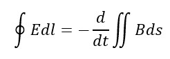
Popularly quoted as “the EMF induced in coil is rate of change of flux through the coil”.
If the right-hand term is forced to zero, we get KVL.
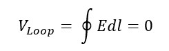
So, whenever we apply KVL to any loop of a circuit we unknowingly set the rate of change of flux linking the circuit to zero, if that is not the case as above, we get wrong answers.
We know for sure that KCL is also a special case of Maxwell Equation, but we by now, are not quite able to manipulate the equations, it would be updated shortly.
You can also write to us.
The Grand Theory of Machines
Very broadly speaking, there exist two types of machines, the machines running on DC Supply and another on the AC Supply. Under the DC category, we have shunt, series, compounded motors, under AC category we have Induction horses, Cylindrical Synchronous and Salient Synchronous machines. Other machines like BLDC, Stepper, SRM are extension of these basic machines only. It takes over two semesters to get all of them in our heads, and that to just vaguely.
Nearly all the important calculations on DC Machines can be made by three simple equations.

![]()

All the engineering relevant parameter of an Induction Motors can be deduced by drawing the equivalent circuit.

This simple diagram all the details the rotor speed (if synchronous speed is known), the current, power factor, the core loss, the air-gap power, the rotor copper loss, the mechanical power and the torque.
For Synchronous Machine we usually draw phasors to get all-important numbers like Torque, power, current, power factor.
Dropping down all the details of how the machine works almost all numerical can be solved out if one remembers the equations, equivalent circuit and phasors as mentioned above.
But it becomes tricky when one tries to explain them, as for different machines we have to follow different approaches to explain the generation of forces and so on.
General approaches are:
The DC motors rotate as current wire experience a force in a magnetic field, Induction Motors runs by virtue of the principle of Electromagnetic Induction, and Synchronous motor runs as rotor field gets locked with the stator field.
We know you would have squeezed your eyebrows as you walked through this paragraph.
There may be several lines along which they may be unified, but here we present our own speculation to understand and explain the operation of all kinds of motors using one single theory.
Basically, the force generated in all the motors (DC or AC) is analogous to force experienced by a magnetic dipole in a magnetic field, trying to align along it. Theoretically, if the angular position in space is stationary or both moving but stationary to each other, then the torque will be constant.
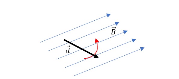
Notice that for given magnitude of the vectors the forces depend on the angle between them, maximizing at 90-degrees.
In DC motors the field produced by stator is fixed in one direction, the rotor though rotating using the help of brushes maintain the current distribution at any angular position in space fixed, irrespective of which conductor coincide at that position it always carries same current in same direction, thus giving rise to another magnetic field (or we shall say dipole) which also remains fixed in space at 90-deg. It is these two dipoles which generate torque and make the rotor rotate.

Induction Machines doesn’t seem to work on this analogy in any way.
Well, let us check.
So, the stator produces a rotating magnetic field at a fixed synchronous speed, meanwhile, the rotor rotates at speed somewhat less than synchronous speed, depending upon the load on the shaft, or depending on slip “s” as we say. Speed of rotating magnetic field of rotor is sNs wrt to rotor structure, this structure is itself rotating with a speed Nr, so the speed of rotor field as seen by the stator field is sNs + Nr- Ns i.e. is luckily zero, hence again we can explain the torque on the rotor by the interaction of two moving magnetic vectors but fixed relatively.
In Synchronous Machines, it’s easily identifiable that field produced by the rotor is fixed wrt to rotor structure but rotates at synchronous speed wrt stator as rotor itself rotates mechanically at synchronous speed. The other field produced by a balanced stator is obviously rotating at synchronous speed, thus again allowing us to imagine torque on the rotor due to interaction of fixed magnetic field and a dipole.
That gives us the freedom to explain the working of all those machines in one shot-one go.
We are also trying this theory to get around Vector Control of Induction motor.
We haven’t figured out but we wonder if similar analogy could also be applied to BLDC, SRM and Stepper too!
Until now we were uniting all the machines to understand the rotating machines as a whole, now let’s divide them.
And when we try to divide them, basically we are entering a domain called Electrical Drives System, in which clear and very sharp boundaries are drawn to distinctly identify the machines for their purposeful use in a given required operation.
Almost all the major subjects of electrical engineering come under the umbrella of electrical drives. Obviously, the machines itself, power electronics for proper power conditioning, control systems for power electronics, the analog and digital electronics for control systems, and lastly the microprocessor for making those electronics alive.
The DC though provide easy speed control, but the problem of sparks and heavy maintenance makes them unfavourable.
The Induction Motor being a very simple, rugged, cheap device and sparkless operation makes them suitable for almost 75% industrial applications today. The bottleneck of Induction Machine is its inherent characteristics to draw reactive power from mains. At higher power levels power factor becomes a crucial parameter as it greatly affects the efficiency, motor heating, overall power system overloading, drop in supply lines, etc.
A higher power rating synchronous motor with god-like control over the power factor is an obvious choice. Not just UPF it can be made to operate at leading power factor, thus balancing the reactive power requirement of industrial setup as a whole.
The Power Flow Equation
Consider a very generalized two-port network. Using KVL we can figure out the current and hence the active and reactive power flow at both sides.

 The apparent power at receiving end:
![]()
As a power system subject always tends to neglect resistances, so the active power can be approximated to:

And the reactive power can be simplified by assuming δ small:
These two equations apply for transmission lines, synchronous motors and generators as well, and are very prominent equation in EE.
Assuming the bus to which synchronous generator is infinite bus, this real power equation becomes useful in the swing curve and is used to study the steady state and transient stability of the gens.
We will see how it is useful in transmission line.
This equation (1) indicates that the direction of power flow is determined by the delta angle (commonly called power angle) and it worth noting that the power flow can occur from to low voltage to high voltage level too, if delta allows.
The equation (2) indicates towards a very crucial phenomenon in transmission line. If the Reactive power is more than there will be more drop in voltage, and conversely more voltage sag indicates towards more reactive power being extracted. Transmission lines being a very high voltage system hence the Voltage Regulation of 5-8% is required, so a strict control of Q is desired.
Moreover, the reactive component of current would cause an unnecessary ohmic loss in long lines as well as underutilization of every component. Reactive power rather than being supplied from generating station it is good to provide it locally hence distribution station began switching their capacitor backs when such voltage sags occur.

The Indispensable Control Theory
Control Theory is about dealing with disturbances which is the absolute nature of nature anyways.
If we had known for sure the response of any system for given input then achieving any desired output would haven’t been much difficult.
For example, if you know for sure person will slap you back if you slap him first, then it won’t be a difficult task to get oneself slapped. The catch is “surety is not there”, he might forgive if he is in a good mood you or even give you a headshot if annoyed, at worse.
Control theory largely accounts for the disturbance, how to still maintain the desired output even under any uncertain disturbances.
All the parameters on which we judge the system performance like fast settling time, less steady-state error can be easily achieved with a suitable controller in an open loop. Close loop, on the other hand, creates stability issues to most of the stable plants, brings the problem of sensor noise, but the greatest advantage is that it takes into account the disturbances (changes in plant models, or externals disturbances, etc.), which becomes of extreme interest in a natural environment.
Power System is a dynamic system, by that we mean it keeps on changing all the time. The tremendous amount of energy that is being generated should always be equal to the energy consumed at any instant because there is no storage in between. Thousands of generators are just only spun and excited to just exactly meet the load demand of millions of consumers spread over a vast geographical area.
This is a huge challenge if we think more deeply.
If we had known exactly the load demand (say 10 W) and we know the loss in lines (say 2 W) and generator losses (say 0.01 W) then we would have calculated the exact rate at which we should fire the coal and we are done and have gone out to play soccer.
Problem is that 10 W never settles. Every time we turn-on even a light bulb the power system adjusts itself to a new equilibrium state.
The pressing of a switch, falling of a tree on lines, or falling of electric poles itself etc. are all different types of disturbances and fixed safe level of parameters like voltages and frequency are desired output of the system, with input being the coal fire rate or diesel-burning rate, or watergate opening, etc. Without feedbacks, we can never do that. Though it’s not like there is just one feedback going back to power stations from the load centres, control system exists at all levels, and it leads to the overall system working as if it were a one close loop. Hence studying Control Systems and Theory becomes of extreme utility to us.
How would we do that will unravel the need to study Analog Electronics, Digital Electronics and Microprocessor and Microcontroller Systems carefully.
The Leverages of Power Electronics
One of the leading reasons why Edison lost to Nikola Tesla in the war of current was the inability to manipulate the DC unlike AC power whose voltage levels could be pushed to extremely high levels with easy by the use of transformers and thereby improving the efficiency and performance of whole power system, leading to the concept of centralization and utilizing the economy of scale.
DC systems like DC motors and DC transmission lines, were hence largely suppressed as the growth of AC accelerated, but they do have their own advantages. And now with hacks of power electronics, DC systems are now gaining ground as complementary to AC systems.
Let us illustrate by a few examples where AC systems have bottleneck and the power electronics comes for their rescue.
Case 1: Power flow in AC lines
The limit on maximum power transfer through a line is the thermal limit and dielectric limit, if the system is already at ultra-high voltage levels then thermal limit becomes the ultimate limit.
So, what we can do to achieve the maximum transferable power.
Voltage levels are raised to dielectric failure, Delta we cannot increase beyond 30-degree. So, the only controllable parameter in our hands in line impedance.
To achieve that max limit decreasing the line impedance is only at our disposal, if there is no control over line impedance then the power lines will be greatly underutilized.
Power electronics allows us for a clean, simple stepless control of effective line impedance, called the series compensation.
Not only that PE now has matured enough to DC manoeuvrings at extraordinarily high voltage and current levels, which enables the concept like HVDC lines that has extremely desirable properties of easy power control.
The direction of power flow was dependent on delta angle, and there is not too much freedom in manipulating this angle nor it is easy it light of stability problems.
HVDC however doesn’t suffer from this issue.
Follow this ABB Hitachi Power Grid commercial advertisement on how the HVDC was only capable to do what they did.
Case 2: Speed Control Problem in Induction Motors
DC Motors were predicted to become obsolete by the end of 1960s but one can see them alive, in fact quite prosperously.
Why?
It has very desirable operating characteristics.
For shunts motors, if torque demand increases so armature current would be increased proportionally if the terminal voltage is kept fixed the change in current would not affect E much as small armature resistance diminishes the effect. Hence speed remains almost constant.
If we want a higher rotor speed, we just simply decrease the field flux.
If we want to operate in a lower speed range, we decrease the supply voltage.
Notice y appropriately changing the parameters many desired characteristics can e obtained.
However, for induction machines, one doesn’t have such a degree of freedom.
Ones a machine is designed its maximum slip gets fixed. Obviously, the maximum slip would be kept low for better efficiency. So its rotor RPM gets limited to a very narrow range. Beyond this limit, the machine would be unstable as we know.
So, we can get a great range of torque for almost constant speed. But varied speed operation is abandoned.
Power Electronics has helped overcome the speed control problems of Induction machines and synchronous machines with the advent of VFDs and other advanced scheme called vector control which almost transforms an Induction Machine to a DC Shunt Motor.
The Torque speed characteristic can be squeezed or expanded by varying the frequency and taking care of supply voltage as other saturation problems or insulation kicks in.
Only at the mercy of power electronics, those drives could be built.
And this list is getting larger and larger every day where power electronics somehow imparts the most favourable characteristics of DC systems to AC systems.
Well devices used in “Power Electronics” called power diodes, power transistors, power MOSFETS, IGBT, don’t differ from “Electronics” counterpart in terms of what they do, however, a simple diode has two layers p and n but power diode have three, so along with having power in front of their names power electronics devices vary greatly in construction.
To be continued………….
NOTE: All the statement made in this blog are authors own mere speculations it may be wrong, so an active reading is greatly expected. Don’t’ keep the statements until you yourself get sure of validity.
Be Critical, Be a CEV!