
“Do you have the courage to make every single possible mistake, before you get it all-right?”
-Albert Einstein
**Featured image courtesy: Internet
THE PROJECT IN SHORT: What this is about?
The importance of analyzing harmonics has been enough stressed upon in the previous blog, Pollution in Power Systems.
So, we set out to design a system for real-time monitoring of voltage and current waveforms associated with a typical non-linear load. Our aim was “to obtain the shape of waveforms plus apply some mathematical rigour to get the harmonic spectrum of the waveforms”.
THE IDEA: How it works?
Clearly, real-time capabilities of any system are analogous to deployment of intelligent microcontrollers to perform the tasks and since this system also demanded some effective visualization setup, so we linked the microcontroller with the desktop (interfacing aided by MATLAB). Together with MATLAB, we established a GUI platform to interact with user to get the required results:
- The shape of waveforms and defined parameters readings,
- Harmonic spectrum in the frequency domain.
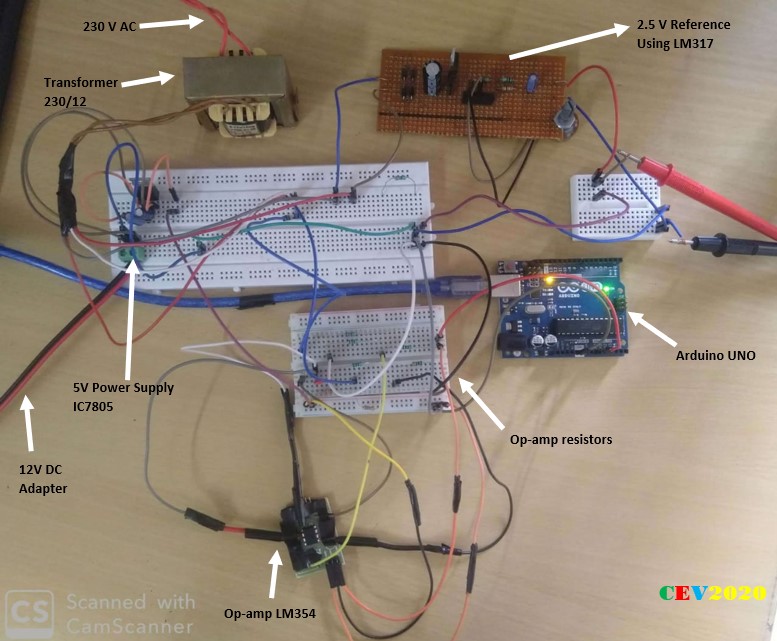
The voltage and current signal are first appropriately sampled by different resistor configurations, these samples are then conditioned by analog industry’s workhorses, the op-amps, and are fed into the ADC of microcontroller (Arduino UNO) for digital discretization. These digital values are accessed by MatLab to apply mathematical techniques according to commands entered by user at the GUI to finally produce required outcome on screen of PC.

ARDUINO and MATLAB INTERFACING: Boosting the Computation
Arduino UNO is 32K flash memory and 2K SRAM microcontroller which sets limit to the functionality of a larger system to some extent. Interfacing the microcontroller with a PC not only allows increased computational capability but more importantly it serves with an effective visual tool of screen to display the waveforms of the quantities graphically, import data and save for future reference and so on.
TWO WAYS TO WORK: Simulink and the .m
The interfacing can be done via two modes, one is directly building simulation models in Simulink by using blocks from the Arduino library and second is to write scripts (code in .m file) in MatLab by including a specific set of libraries for given Arduino devices (UNO, NANO, etc.).
Only the global variable “arduino” needs to be declared in the program and rest codes are as usual and normal. We have used the second method as it was more suitable for the type of mathematical operation we wanted to perform.
NOTE:
- The first method could also be utilised by executing the required mathematical operation using available blocks in the library.
- Both of these methods of interfacing require addition of two different libraries.
THE GUI: User friendly
Using Arduino interfaced with PC also gives another advantage of user-interactive analyzer. Sometimes the visual graphics of waveform distortion is important and sometimes the information in frequency domain is of utmost concern. Using a GUI platform provided by MatLab, to give the option to user to select his choice adds greatly to the flexibility of analyzer.
The GUI platform appears like this upon running the program.

MatLab gives you a very user-friendly environment to build such useful GUI. Type guide in command window select the blank GUI and you are ready to go.
Moreover, you can follow this short 8 minutes tutorial for the introduction, by official MatLab YouTube channel:
REAL-TIME PROGRAM: The Core of the System
Once GUI is designed and saved, a corresponding m-file is automatically generated by the MatLab. This m-file contains the well-structured codes as well as illustrative comments to show how to program further. The GUI is now ready to be impregnated with the pumping heart of the project, the real codes.
COLLECTING DATA
The very first task is to start collecting data-points flushing-in from the ADC of the microcontroller and save it in an array for future reproduction in the program. This should be executed upon the user pressing the START button at the GUI.
Algorithm:
Since we have shifted our whole signal waveform by 2.5 V so we have to continuously check for 127 level which is actually the zero-crossing point, and then only start collecting data.
Code:
% --- Executes on button press in start.
function start_Callback(hObject, eventdata, handles)
% hObject    handle to start (see GCBO)
% eventdata  reserved - to be defined in a future version of MATLAB
% handles    structure with handles and user data (see GUIDATA)
V = zeros(1,201);
time = zeros(1,201);
vstart = 0;
while(vstart == 0)
    value = readVoltage(ard ,'A1');
    if(value > 124 && value < 130)
        vstart = 1;
    end
end

for n = 1:1:201
    value = readVoltage(ard ,'A1');
    value = value – 127;
    V(n) = value;
    time(n) = (n-1)*0.0001;
end
DISPLAYING WAVEFORM
The data-points saved in the array now required to be produced and that too in a way which makes sense to the user, i.e. the graphical plotting.
Algorithm: ISSUES STILL UNRESOLVED!!!
HARMONIC ANALYSIS
As mentioned previously we aimed to obtain the frequency domain analysis for the waveform of concern. The previous blog was presented with insights of mathematical formulation required to do so.
Algorithm: Refer to blog Pollution in power systems
Codes:
% --- Executes on button press in frequencydomain.
function frequencydomain_Callback(hObject, eventdata, handles)
% hObject    handle to frequencydomain (see GCBO)
% eventdata  reserved - to be defined in a future version of MATLAB
% handles    structure with handles and user data (see GUIDATA)

%Ns=no of samples
%a= coeffecient of cosine terms
%b =coefficient of sine terms
%A = coefficient of harmonic terms
%ph=phase angle of harmonic terms wrt fundamental

%a0
sum=0;
n=9   %no of harmonics required
[r,Ns]=size(V);
for i=1:1:Ns
   sum=sum+V(i);
   Adc=sum/Ns;
end


for i=1:1:n
    for j=1:1:Ns
       M(i,j)=V(j)*cos(2*pi*(j-1)*i/Ns);%matrix M has order of n*(Ns)
    end
end


for i=1:1:n
    for j=1:1:Ns
        if j==1 || j==Ns
            sum= sum+M(i,j);
        elseif mod((j-1),3)==0
            sum=sum+ 2*M(i,j);
        else
            sum=sum+3*M(i,j);
        end
    end
   a(i)= 3/4*sum/Ns;
   sum=0;
end

for i=1:1:n
    for j=1:1:Ns
       N(i,j)=V(j)*sin(2*pi*(j-1)*i/Ns);%matrix M has order of n*(Ns+1)
    end
end

for i=1:1:n
    for j=1:1:Ns
        if j==1 || j==Ns
            sum= sum+N(i,j);
        elseif mod((j-1),3)==0
            sum=sum+ 2*N(i,j);
         else
            sum=sum+3*N(i,j);
        end
    end
    b(i)= 3/4*sum/Ns;
    sum=0;
end

for i=1:1:n
    A(i)=sqrt(a(i)^2+b(i)^2);
end

for i=1:1:n
    ph=-atan(b(i)/a(i));
end

figure;
 x = 1:1:n;
 hold on;
 datacursormode on;
 grid on;
 stem(x,A,'filled');
 xlabel('nth harmonic');
 ylabel('amplitude');
CIRCUIT DESIGNING: The Analog Part
The section appears quite late in this documentation but ironically this is the first stage of the system. As we have seen in the power module the constraints on signal input to ADC of microcontroller:
- Peak to peak signal magnitude should be within 5V.
- Voltage Signal must be always positive wrt to the reference.
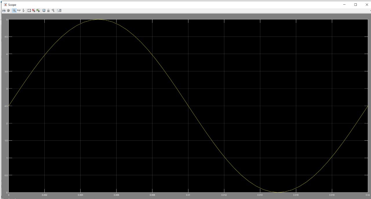
To meet the first part, we used a step-down transformer and a voltage divider resistance branch of required values to get a peak to peak sinusoidal voltage waveform of 5V.
Now current and voltage waveforms obviously would become negative wrt to reference in AC systems.
Think for a second, how to shift this whole cycle above the x-axis.
To achieve this second part, we used an op-amp in clamping configuration to obtain a voltage clamping circuit. We selected op-amp due to their several great operational qualities, like accuracy and simplicity.
Voltage clamping using op-amps:

The circuit overall layout:
IMP NOTE: While taking signals from a voltage divider always keep in mind that no current is drawn from the point of sampling, as it will disturb the effective resistance branch and hence required voltage division won’t be obtained. Always use an op-amp in voltage follower configuration to take samples from the voltage divider.
Current Waveform****(same as power module setup)
MODELLING AND SIMULATIONS:
Now it is always preferable to first model and simulate your circuit and confirming the results to check for any potentially fatal loopholes. It helps save time to correct the errors and saves elements from blowing up during testing.
Modelling and simulation become of great importance for larger and relatively complicated systems, like alternators, transmission lines, other power systems, where you simply cannot afford hit and trial methods to rectify issues in systems. Hence, having an upper hand in this skill of modelling and simulating is of great importance in engineering.
For an analog system, like this, MatLab is perfect. (We found Proteus not showing correct results, however, it is best suited for the simulating microcontrollers-based circuits).

Simulation results confirm a 5V peak to peak signal clamped at 2.5 V.
The real circuit under test:
Case of Emergency:
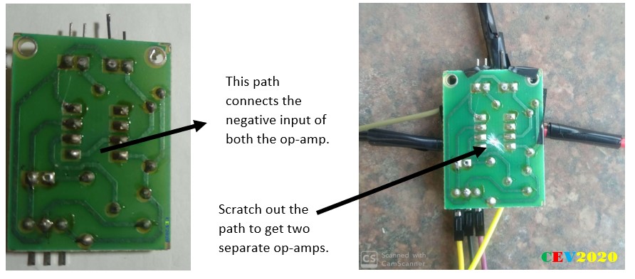
Sometimes we find ourselves in desperate need of some IC and we didn’t get it. At that time our ability to observe might help us get some. In our surroundings, we are littered with IC of all types, and op-amp is one of the most common. Sensors of all types use an op-amp to amplify signals to required values. These IC fixed on the chip can be extracted by de-soldering using solder iron. If that doesn’t seem possible use something that gets you the results. Like in power module project we manage to get three terminals of the one op-amp from IR sensor chip, here we required two op-amps.
First, trace the circuit diagram of the chip by referring the terminals from the datasheet, you can cross-check all connections by using the multimeter in connectivity-check mode. Then use all sorts of techniques too somehow obtain the desired connections.

Reference Voltages
Many times, in circuits different levels of reference voltages are required like 3.3V, 4.5V etc. here we require 2.5 V.
One can-built reference voltage using:
- resistance voltage dividers (with op-amp in voltage follower configuration),
- we can directly use an op-amp to give required gain to any source voltage level,
- the variable reference voltage can be obtained by the variable voltage supply, we built-in rectifier project using the LM317.
WAVEFORM GENERATION
For program testing, we required different typical waveforms like square and triangle wave. These types of waveforms can be obtained in two different ways: the analog way and the digital way.
The Analog Way
Op-amps again come for our rescue. Op-amps when accompanied by resistors, capacitors and inductor seemingly provide all sorts of functionalities in analog domain like summing, subtracting, integrating, differentiating, voltage source, current source, level shifting, etc.
Using a Texas Instrument’s handbook on Op-amp, we obtained the circuit for triangle wave generation as below:
The Digital Way
Another interesting way to obtain all sorts of desired waveforms is by harnessing microcontroller. One can vary the voltage levels, frequency and other waveform parameters directly in the code.
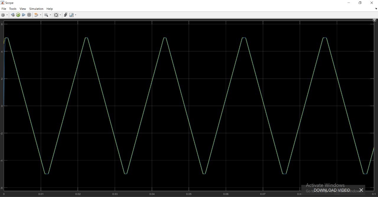
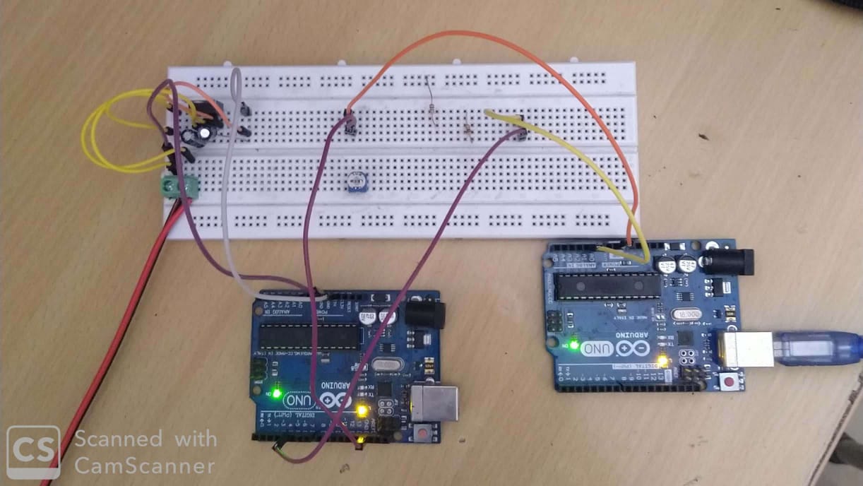
Here we utilised two Arduinos, one stand-alone Arduino 1 which is programmed to generate square wave and another Arduino 2 interfaced with Matlab to check the results.


Now already stated the importance of simulation.
So, here for the simulation of Arduino we used “Proteus 8”.
The code is written in Arduino App, compiled and HEX code is burnt in the model in proteus.

The real-circuit:
The results displayed by the Matlab:

NOTE:
To generate different waveforms other than square-type one thing that has to consider is the PWM mode of operation of Digital pins. The 13 digital pins on Arduino generates PWM.
At 100% duty cycle 5 V is generated at the output terminal.
digitalWrite (PIN, HIGH): This code line generates a PWM of 100% DT whose DC value is 5V.
So, by changing the duty cycle of PWM we can obtain any level between 0-5 V.
analogWrite (PIN, Duty_Ratio): this code line generates a PWM of any duty-ratio (0-100%) hence any desired value of voltage level on a digital pin.
For example:
analogWrite (2, 127): gives an output of 2.5 V at D-pin 2.
Moreover, timer functionalities can be utilized for a triangle wave generation.
THE RESULTS
It is very saddening for us to not able to finally check our results and terminate the project at 75% completion due to unavoidable instances created by this COVID thing.
THE RESOURCES: How you can do it too?
List of the important resources referred in this project:
- MatLab 2020 download: https://www.youtube.com/watch?v=TLAzzxKU5ns
- MatLab official YouTube channel provides great lessons to master MatLab
https://www.youtube.com/channel/UCgdHSFcXvkN6O3NXvif0-pA
- Matlab and Simulink introduction, free self-paced courses by MatLab:
- Simulink simulations demystified for analog circuits: https://www.youtube.com/watch?v=Zw0oiduA70k
- Proteus introduction: https://youtu.be/fK5oI1XfDYI
- MatLab with Arduino: https://youtu.be/7tcEs0QOiBk
- Op-amp cook book: Handbook of Op-amp application, Texas Instruments
THE CONCLUSIONS: Very Important take-away
“TEAMWORK Works”
If we (you and us) desire to take-on venture into the unknown, something never done before and planning to do it all alone, trust our words failure is sure. It gets tough when we get stuck somewhere and it gets tougher only.
We all have to find the people who have the same vision as ours, share some interests and with whom we love work alongside. We all have compulsorily to be a part of a team, otherwise life won’t be easy nor pleasing. There is a great possibility of coming out a winner if we get into it as a team, even if the team fails, we don’t come out frustrated at least.
Each member brings with themselves their own special individual talent to contribute to the common aim. The ability to write codes, the ability to do the math, the ability to simulate, the ability to interpret results, the ability to work on theory and work on intuition, etc. A good teamwork is the recipe to build great things that work.
So, we conclude from the project that teamwork was the most crucial reason for the 75% completion of this venture, and we look forward to make it 100% asap.
Team-members: Vartik Srivastava, Anshuman Jhala, Rahul
Thankyou❤ Ujjwal, Hrishabh, Aman Mishra, Prakash for helping us in resolving software related issues.
WONDER, THINK, CREATE!!
Team CEV