Reading Time: 14 minutes
Introduction
The Non-Sinusoids
What’s the conclusion?
Harmonics
THD and Power Factor
Harmonics Generation: Typical Sources of harmonics
Effects
**Featured image courtesy: Internet
Introduction
If we were in ideal world then we would have all honest people, no global issues of Corona and climate crisis, also gas particles would have negligible volume (ideal gas equation), etc. and in particular in the power systems we would have only sinusoidal voltage and current waveforms. 😅😅
But in this real beautiful world we have bunch of dear dishonest people; thousands die of epidemics, globe becoming hotter and also gas particles have volume similarly having pure sinusoidal waveforms is a luxury and unconceivable feat to be achieved in any large power system.
Prerequisite
We have tried to get launched from very beginning so only a strong will to understand is enough but still we will suggest to once you to go through the power quality blog, it will help develop some important insights.
Electrical Power Quality
Let’s go yoooo!!🤘🤘🤘
Now, why we are talking about shape of waveforms? Well, you will get to know about it by the end on your own, for now let us just tell you that the non-sinusoidal nature of waveform is considered as pollution in electrical power system, effects of which ranges from overheating to whole system ending up in large catastrophes.
Non-sinusoidal waveforms of currents or voltages are polluted waveforms.
But how it can be possible that if voltage implied across some load is sinusoidal but current drawn is non-sinusoidal.
Hint: V= IZ
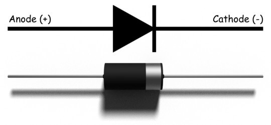
Yes, it is only possible if the impedance plays some tricks. So, the very first conclusion that can be drawn for the systems that create electrical pollution is that they don’t have constant impedance in one time-period of voltage cycle applied across it, hence they draw non-sinusoidal currents from source. These systems are called non-linear loads or elements. Like this most popular guy:

The diode
Note that the inductive and capacitive impedances are frequency variant and remains fixed over a voltage cycle for fixed frequency that’s why resistors, inductor and capacitor are linear loads. In this modern era of 21st century the power system is cursed to be literally littered with these non-linear loads and it is estimated that in next 10-15 years 60% of total load will be non-linear type, well the aftermath of COVID19 has not been considered.
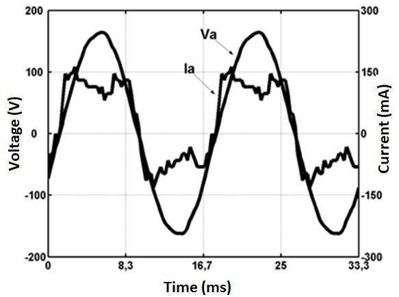
The list of non-linear loads includes almost all the loads you see around you, the gadgets- computers, TVs, music system, LEDs, the battery charging systems, ACs, refrigerators, fluorescent tubes, arc furnaces, etc. Look at the following waveforms of current drawn by some common devices:
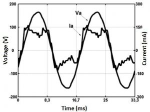
Typical inverter Air-Conditioner current waveform (235.14 V, 1.871 A)
Source: Research Gate
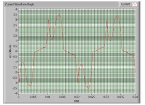
Typical Fluorescent lamp
Source: Internet
Typical 10W LED bulb
Source: Research Gate
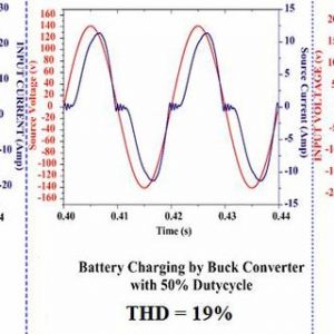
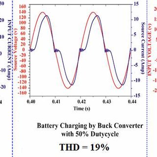
Typical battery charging system
Source: Research Gate
Typical Refrigerator
Source: Research Gate
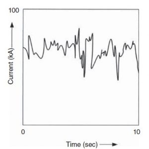
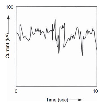
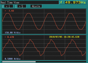
Typical Arc furnace current waveform
Source: Internet
Name any modern device (microwave-oven, washing machine, BLDC fans, etc.) and their current waveforms are severely offbeat from desired sine-type, given the no of such devices the electrical pollution becomes a grave issue for any power system. Now the pollution in electrical power system is not a phenomenon of this 21st century rather electrical engineers have struggled to check the non-sinusoidal waveforms throughout 20th century and one can find description of this phenomenon as early as in 1916 in Steinmetz ground-breaking research paper named “Study of Harmonics in three-phase Power System”. However, the source and reasons of power pollution have ever-changing since then. In early days transformers were major polluting devices now 21st gadgets have taken up that role, but the consequences have remained disastrous.
WAIT, WAIT, WAIT…. What’s that “Harmonics”?
Before we even introduce the harmonics let just apply our mathematical rigor in analyzing the typical non-sinusoidal waveforms, we encounter in the power system.
THE NON-SINOSOIDS
From the blog on Fourier series, we were confronted with one of most fundamental laws of nature:
FOURIER SERIES: Expresssing the alphabets of Mathematics
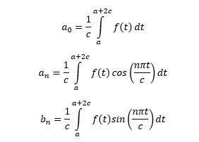
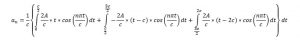
Any continuous, well-defined periodic function f(x) whose period is (a, a+2c) can be expressed as sum of sine and cos and constant components. We call this great universal truth as the Fourier Expansion, mathematically:
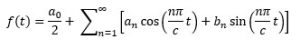 Where,
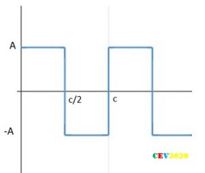
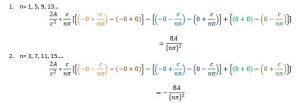
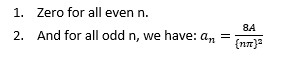
Square-wave, the output of the inverter circuits:
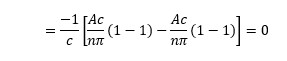
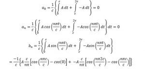 For all even n:
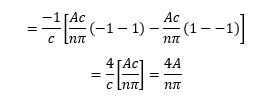
For all odd n:
Just for some minutes hold in mind the result’s outline:
We will draw some very striking conclusions.
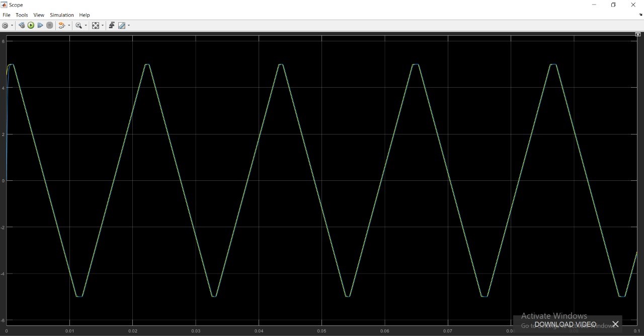
Now consider a triangular wave:
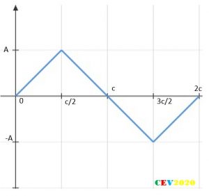
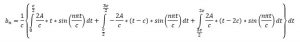
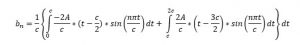
The function can be described as: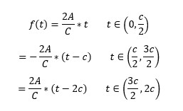
Calculating Fourier coefficients:
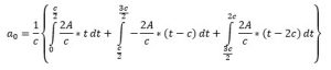
Which again simplifies to zero.
So, we have-
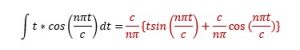
Applying the integration for each interval and putting the limits: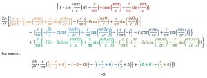
For even n,
=0
For odd n,
=0
😂😂😂
Now,
For even n:
=0
😂😂😂
Are these equations kidding us???
For odd n:
So finally, summary of result for the triangle waveform case is as follows:
Did you noticed that if these two waveforms were traced in negative side of the time axis than they could be produced by:

This property of the waveforms is called the odd symmetry. Since sine wave have this same fundamental property hence only components of sine waves are found in the expansion.
Now consider this waveform:
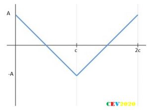
This waveform unlike the previous two cases, if the negative side of waveform had to obtained than it must be:
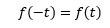
Now this is identified as the even symmetry of waveform, so which components do you expect sine or cos???
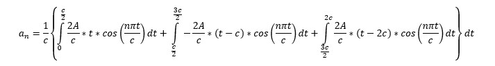
The function can be described as:
 Here again,
 For the cos components:
This equation reduces to:
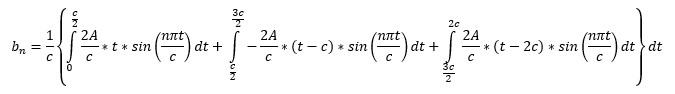
For the sine components:
This equation reduces to Zero for all even and odd “n”.
Well we have guessed it already🤠🤠.
Summary of coefficients for a triangle waveform, which follows even symmetry is as follows: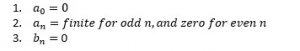
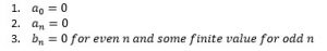
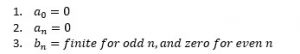
Very useful conclusions:
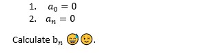
- a0 = 0: for all the waveform which inscribe equal area with x-axis, under negative and positive cycle. This happens because the constant component is simply the algebraic sum of these two areas.
- an = 0: for all the waveform which follows odd symmetry. Cos is an even symmetric functions, it simply can’t be component of a function which is odd symmetric.
- bn = 0: for all the waveform which follows even symmetry. by the same logic sine function which is itself odd symmetric, cannot be component of an even symmetry.
- The fourth very critical conclusion which can be drawn for the waveforms which follow this is:
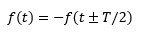
Where T is time period of waveform.
For then the even ordered harmonics aren’t present, only odd orders. This is property is identified as half-wave symmetry, and are present in most power system signals.
Now, these conclusions are applicable to the numerous current waveforms in the power system. Most of the devices with which we have begun with were seemed to follow the above properties, they all are half-symmetric and either odd or even. These conclusions result in great simplification while formulating the Fourier series for power systems waveforms.
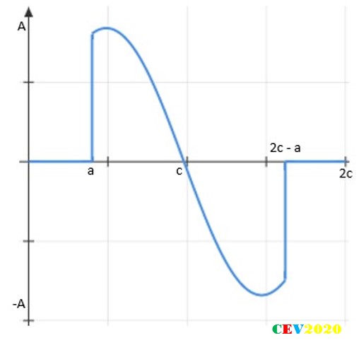
So, consider a typical firing angle Current:
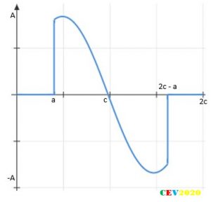
So, apply the conclusions drawn for this case. Since the waveform has no half-wave symmetry but is odd symmetric.
The Harmonics
Hope you had enjoyed utilizing the greatest mathematical tool and amazed to break the intricate waveforms into fundamental sines or cosines.
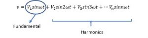
“Like matter is made up of fundamental units called atoms, any periodic waveform consists of fundamental sine and cosine components.”
It is these components of any waveform, which we call in electrical engineering language the Harmonics.
The Mathematics gives you cheat codes to understand and analyze the harmonics. It just simply opens up the whole picture to very minute details.
So, what we are going to do now, after calculating the components, the harmonics?
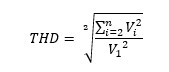
So first all we need to quantify how much harmonic content is present in the waveform. The term coined for this purpose is called total harmonic distortion:
THD, total harmonic distortion:
It is a self-explanatory ratio, the ratio of rms of all harmonics to the rms value of fundamental.
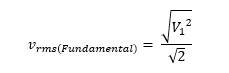
Now since harmonics are sine or cos waves only so the RMS is simply:
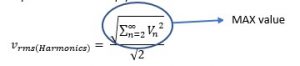
same definition the RMS of fundamental becomes:
So, THD is:
The next thing we are concerned about is power. So, we need to find the impact of harmonics on power transferred.
Power and the Power Factor
The power and power factor are so intimately related. It becomes impossible to talk about power and not of power factor.
So, the conventional power factor definition for any load (linear and non-linear load) is defined as the ratio of active power to the apparent power. It basically is an indicator of how well the load is able to utilize the current it draws; this statement is consistent with statement that a high pf load draws less current for same real power developed.
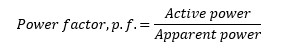
Where
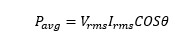
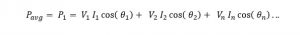
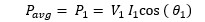
- Active power is: average of instantaneous power over a cycle
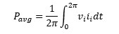
Assuming the sinusoidal current and the voltage have a phase difference of theta, the integration simplifies to:
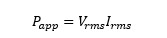
2. Apparent power is by its name simply VI product, since quantities are AC so RMS values.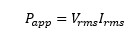
The pf becomes cos(theta), only when waveforms are sinusoidal.
NOTE: The assumption must be kept in mind.
So, what happens when the waveforms are contaminated by harmonics:
There are many theories for defining power when harmonics are considered. Advanced once are very accurate and older once are approximate but are equally insightful.
Let the RMS of the fundamental, first second, the nth component of voltage and current waveform be
The most accepted theory defines instantaneous power as:
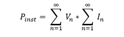
Expanding and integrating over a cycle will cancel all the terms of sin and cos product, and would reduce to:
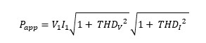
Apparent power remains the same mathematically:
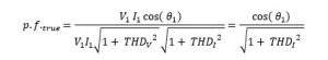
Including the definition of THDs for voltage and current the equation modifies to:
Now this theory uses some important assumptions to simplify the results, which are quite reasonable for particular cases.
- Harmonics contribute negligibly small in active power, so neglecting the higher terms:
2. For most of devices the terminal voltages don’t suffer very high distortions, even though the current may be severely distorted. More on this in next section but for now:
So,
WHAT’S THE CONCLUSION?
The power factor for a non-linear load depends upon two factors, one is cosø and the another is current distortion factor.
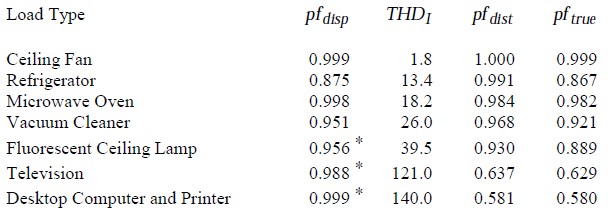
If we wish to draw less current, we need to have high overall power factor. Once cosø component is maximized to one, then distorted current sets the upper limit for the true power factor. Following data accessed by virtue of sciencedirect.com will make it visualize better how much significant the current distortion are.


Notice the awful THD for these devices, clearly, it severely reduces the overall pf.
However, these dinky-pinky household electronics devices are of low power rating so current drawn is not so significant, if they were high powered it would have been a disaster for us.
NOTE: For most of the devices listed above the assumption are solidly valid.
Are you thinking of adding a shunt capacitor across the laptop or the electronic gadgets to improve power factor to get low electric bills, for god sake don’t ever try, your capacitor will be blown in air, later we will understand!!!
These harmonics by a phenomenon of “Harmonic Resonance” with the system and the capacitor banks, amplify horribly. There have been numerous industrial catastrophes that have occurred and still continue to happen because people ignore the Harmonic Resonance.
Our Prof Rakesh Maurya had been involved in solving out one such capacitor bank burn-out issue with Adjustable Speed Drive (ASD) at LnT.
Harmonics Generation: Typical Sources of harmonics
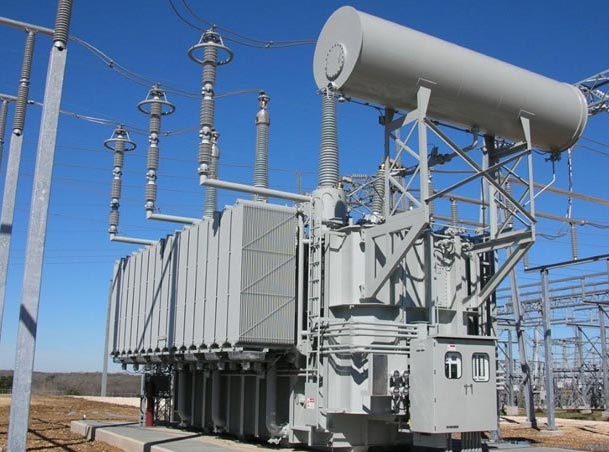
Most of the time in electrical engineering transformers and motors are not visualized as:


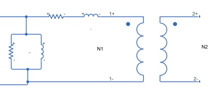
Instead, it is preferred to see transformers and electrical motors like this, respectively:
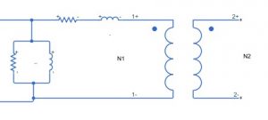
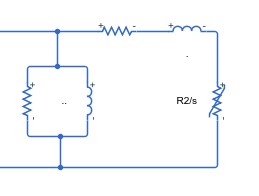
These diagrams are called the equivalent circuits, these models are simply the abstraction developed to let as calculate power flow without considering many unnecessary minute details.
The souls of these models are based on some assumptions which lead us to ignore those minute details, simplify our lives and give results with acceptable error.
Try to recall those assumptions we learned in our classrooms.
The reasons for harmonics generation by these beasts lie in those minute details.
Transformers
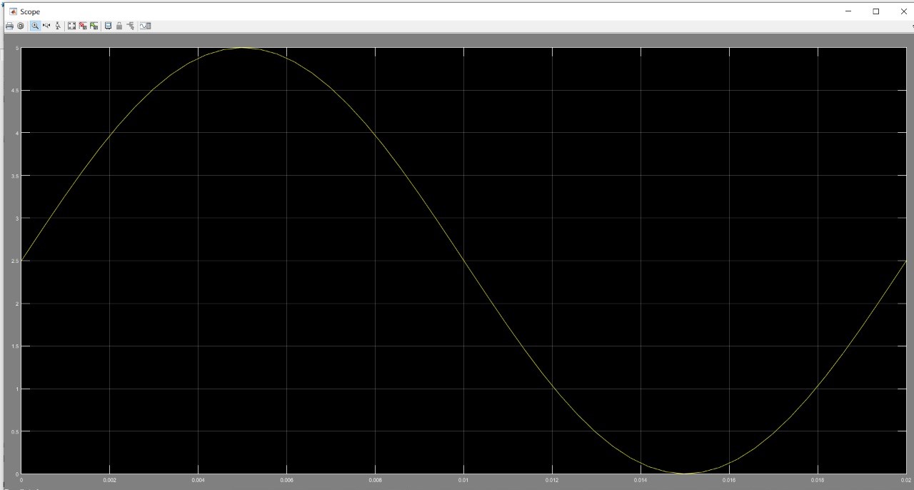
It is only under the assumption of “no saturation” that for a sinusoidal voltage implied across primary gives us sinusoidal voltage at secondary.
Sinusoidal Pri. Voltage >>> Sinusoidal Current >>> Sinusoidal Flux >>> Sinusoidal Induced Sec. EMF
With the advancement in material science now special core materials are available which saturates rarely, but the older and conventional saturated many times and are observed to generated 3rd harmonics majorly.
Details right now are beyond our team’s mental capacity to comprehend.
Electrical Motors
From this stand-point of cute equivalent circuit the electrical motors seem so innocent, simple RL load certainly not capable to introduce any harmonics. But as stated this abstraction is a mere approximation to obtain performance characteristics as fast and reliably as possible.
Remember while deriving the air-gap flux density it was assumed that the spatial distribution of MMF due to balanced winding is sinusoidal, but more accurately it was trapezoidal, only fundamental was considered. Due to this and many other imperfections, motor is observed to produce 5th harmonics, largely.
NOTE: Third harmonics and its multiples are completely absent in three-phase IMs. Refer notes.
Semiconductors
Disgusting, they don’t need any explanation. 😏😏😏
Effects
Power Loss
Most common, however least impactful effect of power harmonics are increased power loss leading to heating and decreased efficiency of the non-linear (devices that causes) and also later we will learn it affects linear devices too, that are connected to the synchronous grid.
The Skin Effect:
Lenz law states that a conducting loop/coil always oppose the change in magnetic flux linked by it, by inducing an emf which leads to a current.
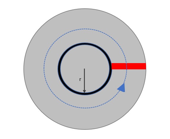
Consider a rectangular two-wire system representing a transmission line having here a circular cross-section wire carrying a DC current I.
Now one loop is quite obviously visible, the big rectangular one. The opposition to change in magnetic field linked by this loop gives us transmission line inductance.
NOTE: THE INDUCTANCE AND LOOPS OF CURRENT ARE FACET OF SAME COIN, ONE LEADS TO ANOTHER. Think about it!!!!
At frequencies relatively higher than power frequency 50 Hz, another kind of current loops begin to magnify. So, as we said this will cause another type of inductance.
Look closely the magnetic field inside the conducting wire is also changing, as a result, inside the conductor itself loops of currents called eddy current set up, which lead to some dramatic impact.
EDDY CURRENT ARE SIMPLY MANIFESTATION OF SIMPLE LENZ LAW, RESPONSE OF A CONDUCTING MATERIAL TO CHANGING MAGNETIC FIELD.
Consider two cases, a current element dx at r and R distance from the center. Which current element will face greater opposition by the eddy currents due their changing nature??
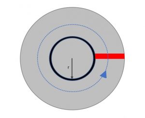
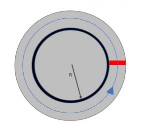
Yes, true, the element lying closer from the center, as the loop area available is more for eddy currents, this difference in opposition from the eddy current to different elements cause the current distribution inside the conductor to shift towards the surface as least eddy current opposition would be there.
A technical account for this skin effect in given in this manner:
- The flux linked by the current flowing at the center region is more than the elements of current at outer region of cross-section;
- Larger flux linkage leads to increased reactance of central area than the periphery;
- Hence current chose the path of least impedance, that is surface region.
Eddy current phenomenon is quite prevalent in AC systems. Since the AC systems are bound to have changing magnetic fields thus eddy currents are induced everywhere from conductors to transformer’s core to the motor’s stator, etc.
Now when higher frequency components of harmonics are present in the current, the skin effect becomes quite magnified, most of the current takes up the surface path as if central region is not available which is equivalent to reduced cross-section i.e. increased resistance, hence magnified joule’s heating (isqR). Thus, heating is increased considerably due these layers on layer reasons (one leads to another).
Other grave effects include false tripping, unexplained failures due to the mysterious harmonic resonance.
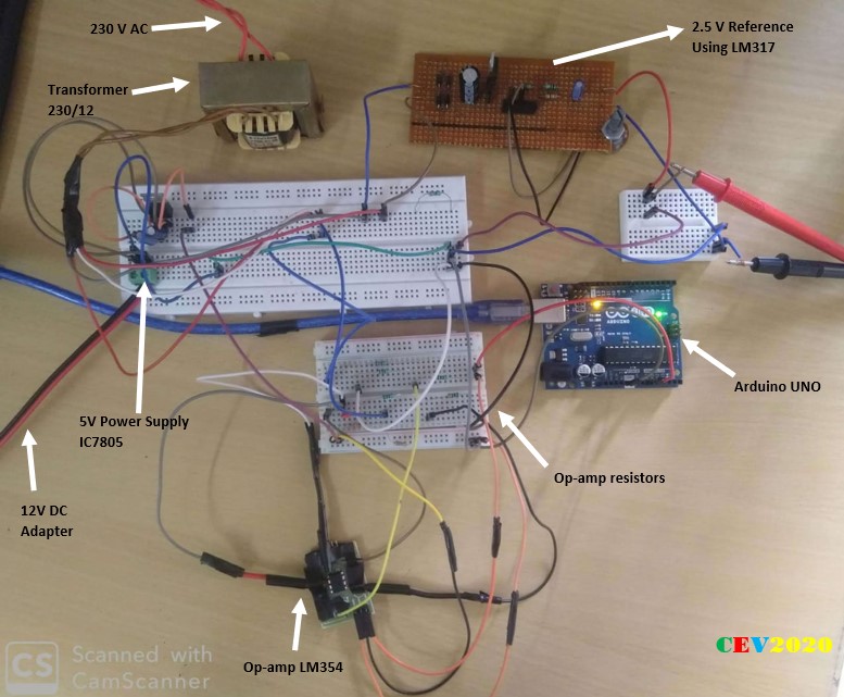
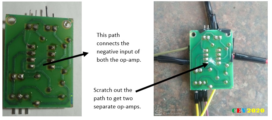
All of these motivated us to build our own harmonic analyzer, follow up the next blog.
Wonder, Think, Create!!!
Team CEV